What do we mean by ‘Statistics’? With an upper-case ‘S’, Statistics is the discipline of systematically analysing data that either consist of numbers or can be represented by numbers. Numerical data are collected in quantitative research studies where the aim is to investigate a research question involving counting or measuring. With a lower-case ‘s’, ‘statistics’ are quantities calculated from data values that tell you something about the data.
For example, as part of their research, Koima et al (2014) wanted to estimate the prevalence of exclusive breastfeeding among HIV-positive women in Nairobi, Kenya. They also wanted to find what factors influenced adherence to exclusive breastfeeding and to measure how strong the relationships were. Such questions can only be addressed using numerical data, which the authors collected using interviewer-administered questionnaires. The authors also collected qualitative data via interviews and focus groups to triangulate with and enrich the quantitative findings.
Statistics involves what appear to be complicated words, concepts and methods, and this may put people off. But part of training to be a midwife involves, to some extent, learning a new language, new ideas and new processes. We need the new language to describe what we are looking at and working with, and to be able to communicate what we find to others. Like other languages, you have to live in the land of Statistics for some time before you can speak it fluently. The first statistical word to be aware of is ‘variable’—an item of information that can vary from one participant to another.
In their study, Koima et al (2014) included variables such as the age of the woman, whether HIV was diagnosed before or during pregnancy, and whether the woman was taught the importance of exclusive breastfeeding. Each of these can vary from participant to participant.
Summarising data using statistics
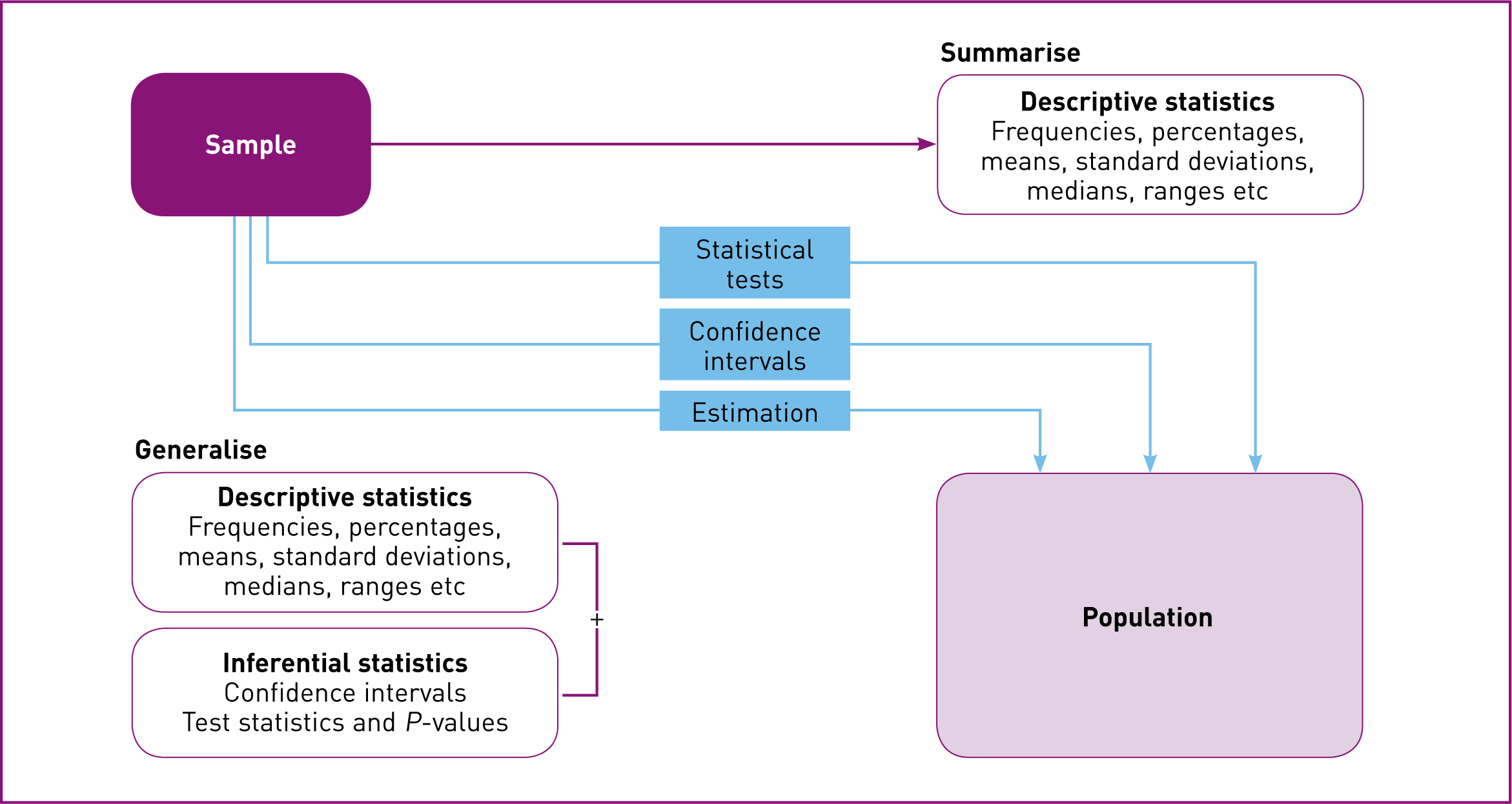
The first task for Statistics is to summarise quantitative data (Figure 1). The tables in Koima et al (2014) summarise details of 22 variables, and undoubtedly many more were collected on their questionnaires for the 188 HIV-positive women. Twenty-two variables for 188 participants gives over 4000 data values, and the authors needed to summarise the information in the data using descriptive statistics. The statistics they used were simple and obvious ones—frequency counts and percentages to summarise the most important details of the participants.

Generalising data using statistics
The second task for Statistics is to generalise quantitative findings. The purpose of a quantitative research study is to find new numerical knowledge, but the new knowledge will have limited use if it cannot be generalised beyond the location, setting and date of the study itself. In Statistics, we generalise using a conceptual framework of populations and samples:
Koima et al (2014) could not collect data from the entire population of HIV-positive women in Nairobi. The study was based at one maternity hospital, and transmission of HIV is an ongoing problem, so the population would be ever-increasing. The authors made a pragmatic compromise to select a sample of HIV-positive women at that hospital within the timeframe of the study, which they hoped would be representative of the population. If the sample is representative, then what we see happening in the sample may be generalised to what might be happening in the population. The descriptive statistics calculated for a sample, like percentages and means, should be good guesses of the corresponding values in the population. If there is no underlying population because of the way the sample was selected—e.g. a purposive sample in a qualitative study—then the descriptive statistics are still valid, but all they do is summarise the sample: they cannot be generalised.
Koima et al (2014) also used confidence intervals to generalise from sample to population. These are ranges of values calculated from the sample that are highly likely to contain the population value. In addition, the authors used statistical tests such as the chi-square test to generalise from sample to population. Such tests assess evidence for or against statements about population values using data from the sample to calculate test statistics. The test approach involves inferential statistics, because we are inferring statistically from sample to population.
Variables
Before we can go ahead with any analysis of quantitative data, we need to decide what kind or kinds of variables we have. The types of variables we have will largely determine how we run the analysis. The language of Statistics has various dialects—concepts or methods sometimes have more than one name. We will illustrate the different types or measurement levels of variables using examples from Akpabio et al (2012), who reported on a study comparing women in Akpabio, Nigeria who preferred either traditional birth attendants (TBAs) or modern health care practitioners for childbirth.
Dichotomous variables
The simplest type of variable is one that only takes two possible values or named categories. This is called dichotomous, or binary: having two named categories. Any variable that takes the values ‘yes’ or ‘no’, ‘present’ or ‘absent’, or ‘true’ or ‘false’ is dichotomous. One of the tables in the study by Akpabio et al (2012) shows eight questions such as ‘TBAs are not as skilled as midwives’ that the respondents answered with either ‘yes’ or ‘no’. These are dichotomous variables.
Nominal variables
The next simplest type is a nominal variable that takes more than two values or named categories, but where there is no natural order present between the categories. In another table in the Akpabio et al (2012) study, marital status (married, never married, separated, widowed, divorced) and religion (Christianity, traditional religion, Islam) are nominal. Each variable has more than two answers, and the categories are not ordered.
Ordinal variables
Moving up a level is an ordinal variable, which also takes more than two values or named categories, but where there is a natural order present between the categories.
Akpabio et al (2012) include a table that shows highest educational level attained (no formal education, primary education, secondary education, tertiary education) and monthly income (N5000–10 000, N11 000–20 000, N21 000–30 000, N31 000–40 000, N41 000–50 000, N51 000–60 000, where N is the Nigerian naira)—these variables are ordinal. Like the previous examples, each variable has more than two answers, but this time the categories are arranged in an increasing order, which may be important for analysis.
Interval/ratio variables
The final types involve variables that take values measured on a numerical scale:
There is a very fine difference between the two types. Interval variables, such as temperature in degrees Celsius, do not have an absolute zero on their scale: 0°C is just an arbitrary point. Indeed, the Swedish astronomer Anders Celsius originally chose the boiling point of water as his ‘zero’. This means than you cannot say that one temperature was so many times higher than another. Ratio variables, such as birth weight, do have an absolute zero, even though it may not occur in practice, so you can say one baby was so many times heavier than another. However, interval and ratio variables can be analysed statistically using the same methods, and for simplicity, they are often considered as a combined type. Akpabio et al (2012) treated two variables, age (years) and parity, as interval/ratio because they reported interval/ratio-type descriptive statistics, which were mean and standard deviation. Maternal age in years is obviously measured on a scale, but parity is an interesting example. Depending on the range of values occurring in a study, parity may be treated as interval/ratio or ordinal, and summarised and analysed in different ways. For example, if you were working with a population of younger women who mostly had yet to give birth or had given birth only once, you might treat parity as ordinal (0, 1, 2 or more).
‘Categorical variables are also, confusingly, called qualitative variables—not because they have anything to do with qualitative research but because they refer to qualities of the participants’
Working with the different types of variables
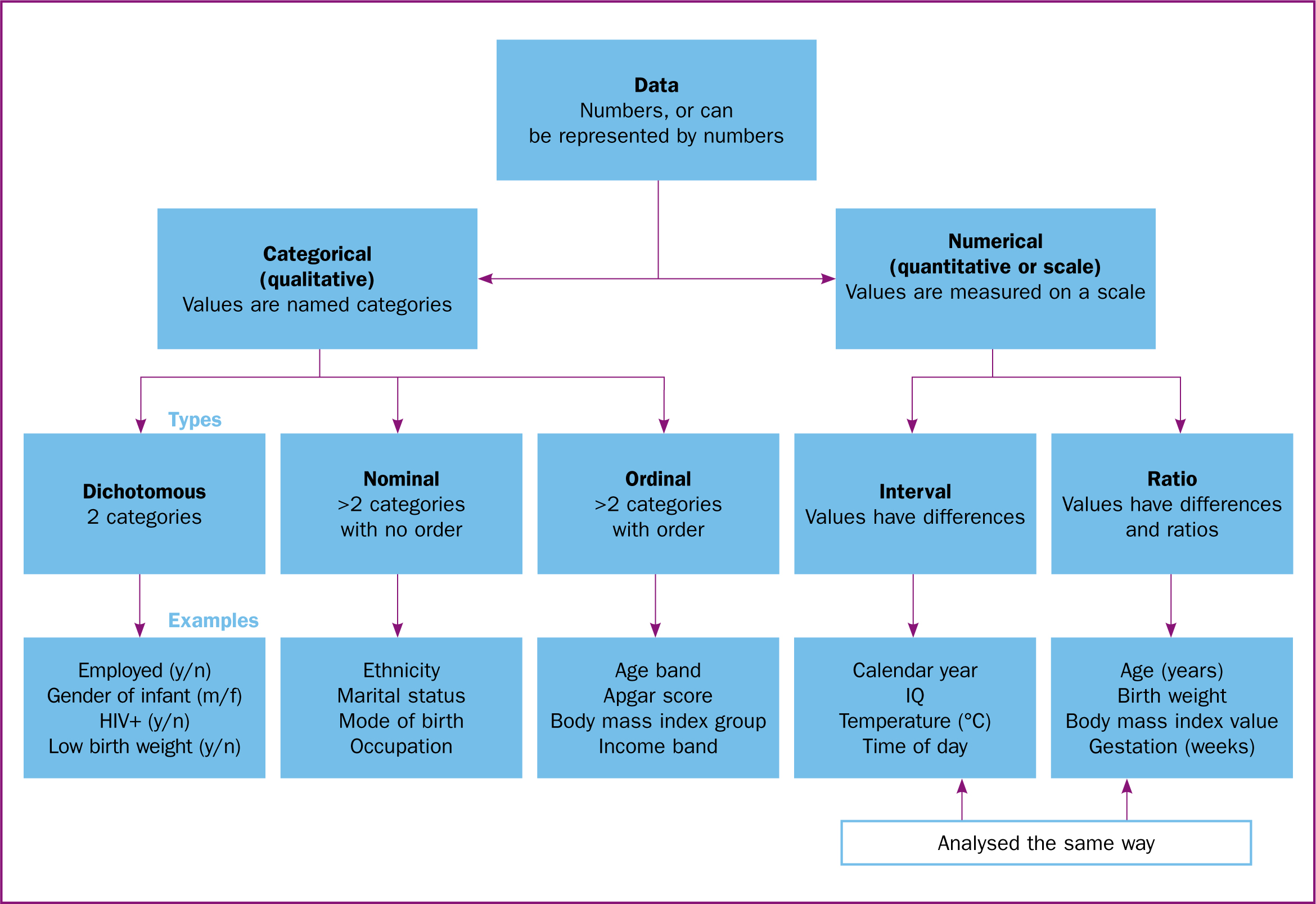
Because they usually refer to categories, dichotomous, nominal and ordinal variables are often called categorical variables (Figure 2). They are also, confusingly, called qualitative variables—not because they have anything to do with qualitative research but because they refer to qualities of the participants, such as occupational status. Interval and ratio variables are also called numerical (as opposed to categorical), scale or quantitative variables, because they refer to measured quantities associated with the participants.

The five types of variables—dichotomous, nominal, ordinal, interval and ratio—are in increasing order of complexity. Nominal is dichotomous but with extra categories, ordinal is nominal with order added, interval is like ordinal with meaningful differences, and ratio is interval with ratios of values. There are different ways of analysing the five types and their combinations. Dichotomous, nominal and ordinal variables are usually summarised by counting how many times the different categories occur, either across the entire sample or within particular groups. Interval and ratio variables can be treated the same way in analysis, and interval/ratio variables are usually summarised using descriptive statistics like means and standard deviations—again, either across the entire sample or within particular groups.
Sometimes it is necessary to analyse a variable that is at a higher level as though it were at a lower level. This can happen when variables such as duration of illness, gestational age and income do not satisfy assumptions required for certain analyses of interval/ratio variables, and instead, we use statistical methods that only depend on ordinal properties. Interval/ratio variables like maternal age in years, income and body mass index are often summarised in ordinal groups because the numbers and percentages are easier to interpret and communicate. This is an important point to remember: in Statistics, there is often more than one way of doing something.

